
【RLchina2022强化学习暑期课】理论课一-机器学习和深度学习基础
参考资料
Classical Machine Learning
Definition by Tom Mitchell(1998):
Machine Learning is the study of algorithms that
- improve their performance P
- at some tasks T
- with experience E
A well-defined learning task is given by <P,T,E>
Programming : 1 + 2 = ?
Machine Learning: 1 + x = 3 ,x =?
Area
Recommender system
Computer vision
E-commerce
Space exploration
Robotics
Information extraction
Social networks
Debugging software
why we need machine learning
- 识别手写数字
- programming的解决方法
- machine learning 的方法,更优秀
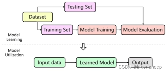
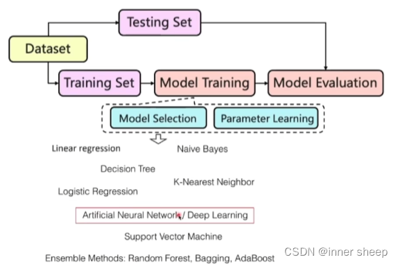
Machine learning workflow
-
Dataset 分为 Training Set 和 Testing Set
-
Model的部署
分为两大部分model 和 Dataset
model
-
Model Training
- Model Selection 确定适合当前任务的模型
- Selection based on human experience
- Linear model for continuous value regression
- Tree-based model for interpretable prediction
- Selection based on learning strategies
- Bayesian optimization
- Bayesian model selection
- Selection based on human experience
- Parameter Learning
- Gradient decent:
- full
- batch
- stochastic
- Gradient decent:
- Model Selection 确定适合当前任务的模型
-
Model Evaluation
-
模型
-
Linear regression
-
Decision Tree
-
Logistic Regression
-
Naive Bayes
-
K-Nearest Neighbor
-
Artificial Neural Network / Deep Learning
-
Support Vector Machine
-
Ensemble Methods:
Random Forset,Bagging,AdaBoost
-
Supervised Learning
- Given a training set (x1,y1),(x2,y2),…,(xn,yn)
- Learn a Function F(x) based on the testing set (xn+1, yn+1),(xn+2,yn+2),…,(xn+m,yn+m).
Linear regression
In linear regression we assume that y and x are related with the following equation:
where w is a parameter
Determine the model parameters
-
Our goal is to estimate w from the training data of (x1,y1),(x2,y2),…,(xn,yn)
-
Optimization goal: minimize squared error (least squares):
\begin{align}min_{w} \sum^{n}_{i = 1} (y_i - wx_i)^2\end{align}
- minimizes squared distance between the true value and predicted value.
- has a nice probabilistic interpretation
-
证明,用偏导数 = 0 解出w
Evaluation of the learned model
learning based on the training set (x1,y1),(x2,y2),…,(xn,yn)
Evaluation based on the testing set (xn+1, yn+1),(xn+2,yn+2),…,(xn+m,yn+m).
-
Root mean squared error(RMSE) 均方根误差
\begin{align} RMSE = \sqrt{\frac{1}{m} \sum^{n+m}_{i = n+1}(y_i - wx_i)^2} \end{align}
-
Mean Absolute Error(MAE) 平均绝对误差
\begin{align} MAE = \frac{1}{m} \sum^{n+m}_{i = n+1}|y_i - wx_i| \end{align}
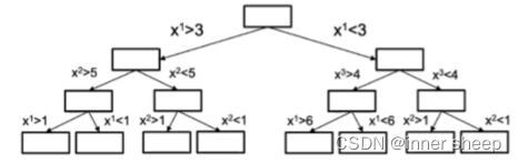
Decision Tree
-
Dataset D= {(x1,y1),(x2,y2),(x3,y3),…(xn,yn)}

举例有以下数列
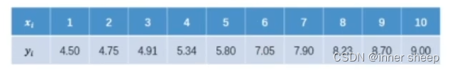
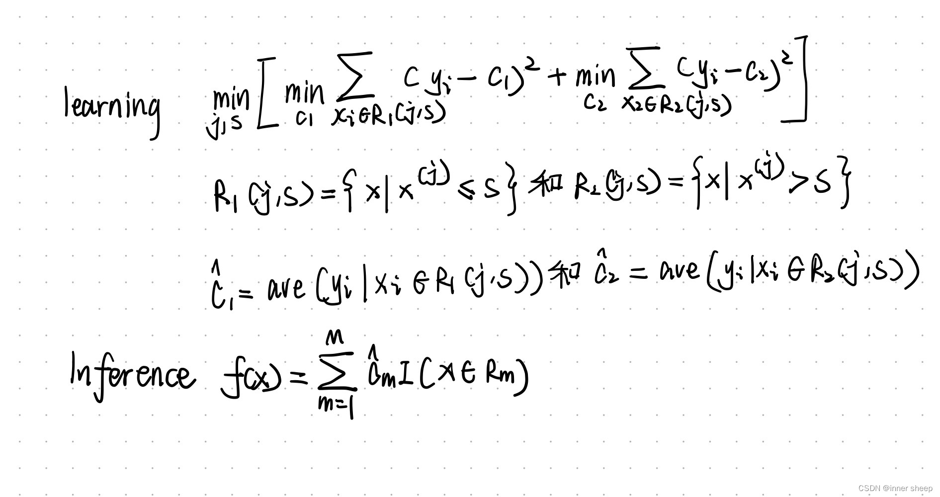
S表示从x1开始划分左右,c1表示左边的平均值,c2表示右边数列的平均值
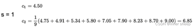
则,得到的c1和c2就是上述公式中的c1和c2,我们可以依次得到所有的可能的S对应的c1和c2,如下表:
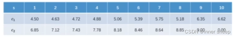
有了所有的c1和c2我们就可以带入公式:

得到如下的表格:
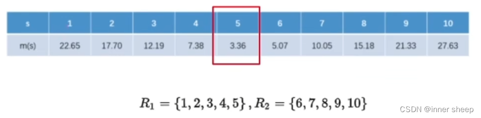
因此我们将m(s)值最小的S = 5,当作分界值
最后我们就生成了一个决策树,大于5往右走,小于5往左走。
Nearest-Neighbor Classifiers
-
Requires three things
- The set of stored records
- Distance Metric to compute distance between records
- The value of K , the number of nearest neighbors to retrieve
-
To classify an unknown record:
- Compute distance to other training records
- Identify k nearest neighbors
- Use class labels of nearest neighbors to determine the class label of unknown record(e.g.,by taking majority vote)
-
Compute distance between two points:
-
Euclidean distance
-
Manhatten distance
-
q norm distance
-
-
Choosing the value of k:
- if k is too small ,sensitive to noise points
- if k is too large ,neighborhood may include points from other classes
-
Determine the class from nearest neighbor list
-
take the majority vote of class labels among the k-nearest neighbors
where is the set of k closest training examples to z.
-
Weigh the vote according to distance
- weight factor,w = $$1/d^2$$
-
Logistic regression
-
The optimal decisions are based on the posterior class probabilities . For binary classification problems, we can write these decisions as
\begin{align}y = 1 \space if \space log\frac{P(y = 1|X)}{P(y=0|X)} > 0 \end{align}
and y = 0 otherwise.
-
We generally don’t know but we can parameterize the possible decisions according to
\begin{align} log\frac{P(y = 1|X)}{P(y=0|X)} =f(x;w) = w_0 + x^T w_1 \end{align}
-
Our log-odds model
\begin{align} log\frac{P(y = 1|X)}{P(y=0|X)} = w_0 + x^T w_1 \end{align}
gives rise to a specific form for the conditional probability over the labels( the logistic model):
\begin{align} P(y = 1|x,w) =g(w_0 + x^T w_1) \end{align}
where
\begin{align} g(z) =(1 + exp(-z))^{-1} \end{align}$$ 激活函数 is a logistic "squashing function " that turns linear predictions into probabilities.
-
As with the linear regression models we can fit the logistic models using the maximum (conditional) log-likelihood criterion.
\begin{align}l(D;w) = \sum_{i=1}^n log P(y_i|x_i,w)\end{align}
where
\begin{align} P(y = 1|x,w) = g(w_0 + x^Tw_1) \end{align}
-
The log-likelihood function $ l(D;w) $ is a jointly concave function of thr parameters w; a number of optimization techniques are available for finding the maximizing parameters.
-
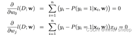
if we set the derivatives of the log-likelihood with respect ot the parameters to zero.
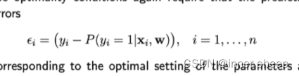
the optimality conditions again require that the prediction errors
corresponding to the optimal setting of the parameters are uncorrelated with any linear function of the inputs.
-
-
testing set 和 Training Set
- 尽量使分布一致
-
Dataset 和 input data
-
How many training samples we need to achieve successful learning
- The learned model can approximate the real model with high probaility
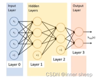
Deep learning
- Multi-layer Perceptron and Back Propagation
-
Multilayer neural networks
-
Both supervised and unsupervised
-
Acitvation functions
- 微信